Geometric aberrations in multiturn operation

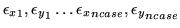
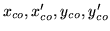
This operation traces particles that are placed on ellipses with nominal emittances $\epsilon_{x_{i}},\ \epsilon_{y_{i}}$ for many turns. It then fits an ellipse to the output points obtained. From this fitted ellipse it determines the average values for
$\beta_{x}, \ \alpha_{x}, \ \beta_{y}, \ \alpha_{y}, \ \nu_{x},\ \nu_{y},\ \epsilon_{x}, and\ \epsilon_{y}$. It also computes the maxima and minima emittances which informs about the diffusion pattern of the motion. Variances of the tunes are also computed.

               Input format 


GEOMetric aberrations .......(up to 80 characters) 

$\beta_{x},\alpha_{x},\beta_{y},\alpha_{y}$ 

$x_{co},x'_{co},y_{co},y'_{co}$,ener 


ncase,nturn,njob 


nplot,nprint 

${\epsilon_{x}}_{1} , {\epsilon_{y}}_{1} \dots {\epsilon_{x}}_{ncase} , {\epsilon_{y}}_{ncase}$ 


anplprt

Parameter definitions

$\beta_{x},\alpha_{x},\beta_{y},\alpha_{y}$

$\parbox{10cm}{ input values of the twiss parameters at the entrance... ...o the first energy are used. This includes the parameters $x_{co}$\ to ener.}$

$x_{co},x'_{co},y_{co},y'_{co}$, ener

$\parbox{10cm}{ coordinates and momentum of the closed orbit around ... ...ement analysis operation. Values corresponding to the first energy are used.}$

ncase $\parbox{10cm}{ number of cases analyzed (maximum mxgaca)}$

nturn $\parbox{10cm}{ number of turns for tracing (maximum 1000)}$

njob

1 $\parbox{10cm}{ coupled motion analysis is wanted}$

2 $\parbox{10cm}{ uncoupled motion analysis is wanted}$

nplot

1 $\parbox{10cm}{ plotting of the resulting particles. The operation ... ...ccumulation at the end of the job. It also computes its own plotting windows.}$

-1 $\parbox{10cm}{ no plotting.}$

nprint

-2 $\parbox{10cm}{ no printing.}$

-1 $\parbox{10cm}{ printing at end of lattice only.}$

0 $\parbox{10cm}{ printing after every element.}$

n $\parbox{10cm}{ printing after every n turns. Normally nprint should be set = nturn.}$

$\epsilon_{x},\ \epsilon_{y}$

$\parbox{10cm}{ ncase values for the chosen nominal emittances in x and y using the unit mm-mrad (E-06 m-rad)}$

anplprt

$\parbox{10cm}{ parameter selecting the fast fourier transform optio... ...rm. Only the first case of the geometric aberration run is fourier analysed.}$

Examples

The first example comes from demo5 and provides an FFT analysis with the plotting of the FFT spectrum but no printout of the spectrum.

The second example, taken from demo12, illustrates how the geometric aberration operation uses the twiss parameters computed in a previous movement analysis operation.

GEOMETRIC ABERRATIONS
2 0 .11 0
0 0 0 0
0
2
1000
1
1 -1
4.5 2.25
9 4.5
110;
stop
* The following is to illustrate the use of rmat and geometric
* aberrations in conjunction with movement analysis
movement analysis
1 1 1 -3 1 0 0.00001
0 0 0 0 0 0.002
0,
geometric aberration
0 0 0 0
0 0 0 0 0
1 100 1
1 -2
10 10,