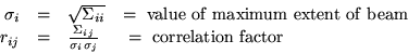
Input formatfollowed by :BEAM matrix tracing.... (up to 80 characters)
![\begin{displaymath}\begin{array}{cccccc}
\sigma _{x}&r_{xp_{x}}&r_{xy}&r_{xp_{y...
...\\
&&&&&\sigma_{\delta} \\
mprint& [mlist]&&&&
\end{array} \end{displaymath}](img52.png)
![\begin{displaymath}\begin{array}{ccccc}
0&&&& \\
\beta_{x}&\alpha_{x}&\eta_{x}&...
...gma_{l}&\sigma_{\delta}&&& \\
mprint& [mlist]&&&
\end{array} \end{displaymath}](img53.png)
![\begin{displaymath}\begin{array}{ccccc}
0&&&& \\
0&0&0&0&\epsilon_{x} \\
0&0...
...gma_{l}&\sigma_{\delta}&&& \\
mprint& [mlist]&&&
\end{array} \end{displaymath}](img54.png)
Parameter definitions
The relationship between the ![]() beam matrix and the input
coefficients is as follows :
beam matrix and the input
coefficients is as follows :
Let ![]() , with
, with ![]() and
and ![]() taking the values
taking the values ![]() ,
, ![]() ,
, ![]() ,
,
![]() ,
, ![]() and
and ![]() , be the elements of the symmetric positive
definite matrix
, be the elements of the symmetric positive
definite matrix ![]() . Then the following formulae describe the
relationship between
. Then the following formulae describe the
relationship between ![]() and the input parameters :
and the input parameters :
![]()
![]()
![]()
![]()
![]() and
and ![]() are the horizontal and vertical
emittances. In this case, the beam is assumed uncoupled .
are the horizontal and vertical
emittances. In this case, the beam is assumed uncoupled .
NOTE :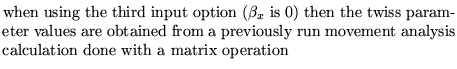
mprint 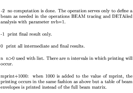
mlist 
Units
![]() are measured in meters
are measured in meters
![]() are
measured in
radians.
are
measured in
radians.
![]() are measured in m-radians.
are measured in m-radians.
![]() unit is one.
unit is one.
The correlation coefficients ![]() are dimensionless and vary
from
are dimensionless and vary
from ![]() to
to ![]()
Examples
Three examples are given. The first is extracted from demo 7 , the second and third are extracted from demo 2.
The first shows the definition of the beam
using the extension ![]() 's.
's.
The second defines the transverse part of the beam by using the twiss parameters and the emittances.
The third shows a definition used in conjunction with a previous matrix analysis. It uses the twiss parameters obtained in that analysis and the value of the tranverse emittances.
BEAM MATRIX TRACING
0.00012157290 0 0 0 0 0
  0.00000246750 0 0 0 0
    0.0000826254 0 0 0
       0.0000036309 0 0
                    0.002 0
                      0.005
-1,

   beam definition
   0
   1.0 0 0 0 1.0e-06
   2.0 0 0 0 1.0e-06
   0.001 0.001
   0,

MATRIX : FIRST ORDER CELL MATRIX.
1 -1,
BEAM MATRIX
0
0 0 0 0 1.0E-06
0 0 0 0 1.0E-06
0.02 0.001
-1;